The ionospheric TEC can be calculated using different delays of two or more transmitted frequencies from the Global Navigation Satellite Systems (GNSS), including GPS. In the GNSS era, the ionospheric TEC provides us an unprecedented opportunity to image the ionosphere plasma content between ground-based receivers and the GNSS satellites. In the recent years, the number of GNSS receivers has increased dramatically and this trend is continuing.
Our TEC map reconstruction model, Video Imputation with SoftImpute, Temporal smoothing and Auxiliary data (VISTA) [Sun et al. 2021], is capable of imputing a time-series of matrices with a large amount of missing values and guarantees both spatial smoothness and temporal consistency, which is very helpful for reconstructing scientific images with non-random missingness, i.e., the TEC maps/videos.
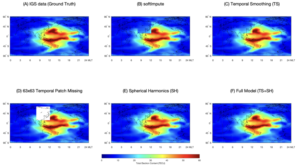
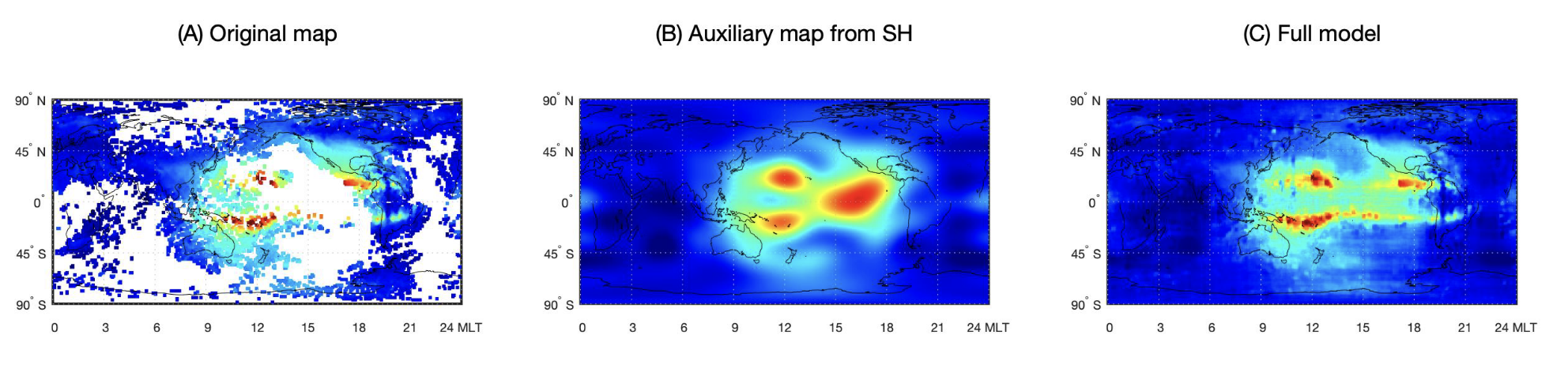
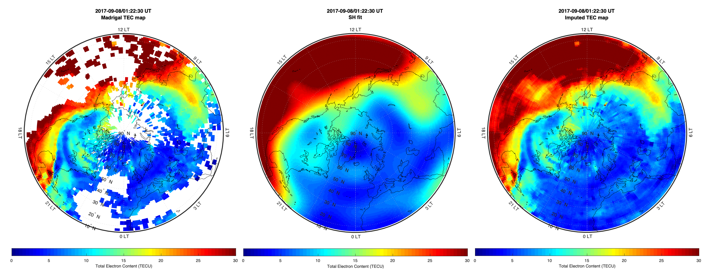
The VISTA method is innovated on top of an existing matrix factorization and imputation completion algorithm, softImpute, with an efficient optimization algorithm. We incorporated auxiliary data, such as spherical harmonic fitted map, and ideas of spatial-temporal smoothness into the existing matrix factorization and imputation model, which results in a novel model that is catered to the special structure of the TEC videos thus giving superior performance for TEC video/map reconstruction. VISTA can not only provide full global-scale maps but also preserve the observed meso-scale ionospheric density structures (e.g., equatorial plasma bubbles, polar cap patch). Examples of applying VISTA to the IGS data with an artificial missing data patch and to the Madrigal TEC data are shown below. More examples can be found in Zou et al., 2021.
We have constructed and completed a global TEC map database using the VISTA algorithm and the database can be accessed freely via UM Deepblue data repository. Description of the database can be found in Sun et al. 2023, including the data processing pipeline, discussions on the computational costs, fine tuning of the VISTA algorithm parameters, and validation of the dataset using independent JASON TEC. Discussions on potential usages of the complete TEC database are given, together with a concrete example of applying this database.